How to tidy Second Spectrum Physical Splits csv files
A walkthrough of the TidySpectrum R Package

Working as a sport scientist requires handling of data from many different external sources. One of these may be from the Second Spectrum, a match video tracking and analytics provider for many major leagues, including the Danish Superliga.
While Second Spectrum provides a basic overview of physical match data across teams and players in the league via their cloud solution, more comprehensive analyses and visualizations require export of the data. Unfortunately, this does not come in a tidy format suitable for analyses, why I saw the need to develop a small R package for transforming the exported csv files into a tidy format to make my life easier.
In this blog post I provide a walk through of the data cleaning and manipulation process of the TidySpectrum package.
A big shout out to the TidyX Screencast by Patrick Ward and Ellis Hughes, who have recorded two excellent videos on how to clean ugly excel files.
Second Spectrum gives access to different physical data files, of which I am most interested in the Physical Splits, which essentially provides 5 minute splits of different running metrics for all players at both teams, including aggregated for each team.
Let us first have a look at the top 50 rows of the csv file as it appear if you import it into R using the read_csv function. In the first few rows you have some meta-data with information on the date and which two teams played each other, followed by some velocity threshold definitions. A few rows later there is an embedded header representing the minute splits followed by TeamA (including metrics) and all players for that particular team (including metrics for each player), and so fourth for TeamB. It is obvious that this is not a data structure/format suited for analyses.
| Second Spectrum Split Data | …2 | …3 | …4 | …5 | …6 | …7 | …8 | …9 | …10 | …11 | …12 | …13 | …14 | …15 | …16 | …17 | …18 | …19 | …20 | …21 | …22 |
|---|---|---|---|---|---|---|---|---|---|---|---|---|---|---|---|---|---|---|---|---|---|
| TeamA - TeamB : 2022-2-21 | NA | NA | NA | NA | NA | NA | NA | NA | NA | NA | NA | NA | NA | NA | NA | NA | NA | NA | NA | NA | NA |
| 02f1d5a7-7ac5-4419-b4ba-85da99a08241 | NA | NA | NA | NA | NA | NA | NA | NA | NA | NA | NA | NA | NA | NA | NA | NA | NA | NA | NA | NA | NA |
| NA | NA | NA | NA | NA | NA | NA | NA | NA | NA | NA | NA | NA | NA | NA | NA | NA | NA | NA | NA | NA | NA |
| Threshold key (km/h) | NA | NA | NA | NA | NA | NA | NA | NA | NA | NA | NA | NA | NA | NA | NA | NA | NA | NA | NA | NA | NA |
| Walking : 7 | NA | NA | NA | NA | NA | NA | NA | NA | NA | NA | NA | NA | NA | NA | NA | NA | NA | NA | NA | NA | NA |
| Jogging : 15 | NA | NA | NA | NA | NA | NA | NA | NA | NA | NA | NA | NA | NA | NA | NA | NA | NA | NA | NA | NA | NA |
| LowSpeedRunning : 20 | NA | NA | NA | NA | NA | NA | NA | NA | NA | NA | NA | NA | NA | NA | NA | NA | NA | NA | NA | NA | NA |
| HighSpeedRunning : 25 | NA | NA | NA | NA | NA | NA | NA | NA | NA | NA | NA | NA | NA | NA | NA | NA | NA | NA | NA | NA | NA |
| LowSpeedSprinting : >25 | NA | NA | NA | NA | NA | NA | NA | NA | NA | NA | NA | NA | NA | NA | NA | NA | NA | NA | NA | NA | NA |
| NA | NA | NA | NA | NA | NA | NA | NA | NA | NA | NA | NA | NA | NA | NA | NA | NA | NA | NA | NA | NA | NA |
| NA | NA | NA | NA | NA | NA | NA | NA | NA | NA | NA | NA | NA | NA | NA | NA | NA | NA | NA | NA | NA | NA |
| NA | NA | NA | NA | NA | NA | NA | NA | NA | NA | NA | NA | NA | NA | NA | NA | NA | NA | NA | NA | NA | NA |
| Minute Splits | 5.00 | 10.00 | 15.00 | 20.00 | 25.00 | 30.00 | 35.00 | 40.00 | 45.00 | 50.00 | NA | 50.00 | 55.00 | 60.00 | 65.00 | 70.00 | 75.00 | 80.00 | 85.00 | 90.00 | 95.00 |
| Team A (62da2c6c-67c5-4478-bcda-34aa58075367) | NA | NA | NA | NA | NA | NA | NA | NA | NA | NA | NA | NA | NA | NA | NA | NA | NA | NA | NA | NA | NA |
| Total Distance | 5055.29 | 6226.41 | 4779.51 | 6256.74 | 6158.10 | 6707.47 | 4424.53 | 6307.07 | 6533.86 | 5019.99 | NA | 6221.51 | 4411.40 | 6702.67 | 6702.17 | 3918.89 | 6728.53 | 4948.54 | 6567.48 | 5974.13 | 5178.85 |
| Walking Distance | 1810.76 | 1799.77 | 1716.37 | 1763.50 | 2013.92 | 1839.54 | 1450.40 | 1807.72 | 1706.15 | 1742.10 | NA | 1812.52 | 1490.97 | 1605.79 | 2010.53 | 1472.90 | 1852.09 | 1841.09 | 1791.84 | 2010.96 | 1530.23 |
| Jogging Distance | 2251.22 | 2555.79 | 1765.35 | 3319.02 | 2872.70 | 3550.96 | 1857.71 | 3200.36 | 2922.58 | 2479.05 | NA | 3102.82 | 1797.89 | 3567.68 | 3217.58 | 1440.42 | 3332.68 | 2048.26 | 3040.14 | 2813.82 | 2557.16 |
| Low Speed Running Distance | 639.64 | 1158.39 | 829.90 | 911.66 | 886.54 | 971.75 | 750.81 | 917.89 | 1209.04 | 664.32 | NA | 929.80 | 595.84 | 1149.67 | 995.77 | 683.30 | 1029.11 | 824.01 | 1082.39 | 699.21 | 692.46 |
| High Speed Running Distance | 255.56 | 540.33 | 347.24 | 228.39 | 279.01 | 317.04 | 317.76 | 307.93 | 582.44 | 123.59 | NA | 292.96 | 411.97 | 357.26 | 414.37 | 240.99 | 388.81 | 192.32 | 542.70 | 297.36 | 336.63 |
| Sprinting Distance | 98.11 | 172.13 | 120.65 | 34.16 | 105.93 | 28.18 | 47.84 | 73.17 | 113.65 | 10.92 | NA | 83.41 | 114.74 | 22.27 | 63.92 | 81.28 | 125.84 | 42.86 | 110.42 | 152.79 | 62.36 |
| Walking Count | 166.00 | 183.00 | 138.00 | 247.00 | 223.00 | 252.00 | 140.00 | 234.00 | 188.00 | 187.00 | NA | 251.00 | 134.00 | 221.00 | 241.00 | 116.00 | 241.00 | 151.00 | 231.00 | 203.00 | 188.00 |
| Jogging Count | 214.00 | 258.00 | 184.00 | 286.00 | 294.00 | 319.00 | 192.00 | 315.00 | 265.00 | 243.00 | NA | 332.00 | 181.00 | 304.00 | 323.00 | 164.00 | 316.00 | 209.00 | 302.00 | 266.00 | 247.00 |
| Low Speed Running Count | 79.00 | 128.00 | 82.00 | 99.00 | 103.00 | 111.00 | 79.00 | 113.00 | 132.00 | 73.00 | NA | 117.00 | 79.00 | 123.00 | 118.00 | 74.00 | 114.00 | 86.00 | 117.00 | 90.00 | 95.00 |
| High Speed Running Count | 28.00 | 45.00 | 30.00 | 20.00 | 28.00 | 30.00 | 22.00 | 28.00 | 50.00 | 11.00 | NA | 28.00 | 31.00 | 35.00 | 31.00 | 22.00 | 35.00 | 20.00 | 40.00 | 27.00 | 31.00 |
| Sprinting Count | 6.00 | 6.00 | 8.00 | 3.00 | 7.00 | 2.00 | 3.00 | 6.00 | 10.00 | 1.00 | NA | 5.00 | 9.00 | 3.00 | 6.00 | 5.00 | 6.00 | 4.00 | 8.00 | 8.00 | 5.00 |
| NA | NA | NA | NA | NA | NA | NA | NA | NA | NA | NA | NA | NA | NA | NA | NA | NA | NA | NA | NA | NA | NA |
| Athlete 1 (9ca4a299-6133-4cb3-aded-8ee19cfe8ced) | NA | NA | NA | NA | NA | NA | NA | NA | NA | NA | NA | NA | NA | NA | NA | NA | NA | NA | NA | NA | NA |
| Total Distance | 433.76 | 538.12 | 380.62 | 527.54 | 539.11 | 640.61 | 327.68 | 582.58 | 540.16 | 431.45 | NA | 570.49 | 359.90 | 396.15 | 607.79 | 82.39 | 0.00 | 0.00 | 0.00 | 0.00 | 0.00 |
| Walking Distance | 165.73 | 154.93 | 149.48 | 142.57 | 216.99 | 169.90 | 140.99 | 177.97 | 149.98 | 186.81 | NA | 165.85 | 150.04 | 123.44 | 176.54 | 19.55 | 0.00 | 0.00 | 0.00 | 0.00 | 0.00 |
| Jogging Distance | 199.77 | 233.12 | 110.25 | 321.39 | 235.03 | 362.28 | 150.64 | 327.54 | 229.87 | 234.11 | NA | 312.86 | 128.82 | 174.69 | 309.65 | 52.89 | 0.00 | 0.00 | 0.00 | 0.00 | 0.00 |
| Low Speed Running Distance | 49.12 | 92.30 | 60.03 | 58.95 | 62.20 | 73.11 | 24.11 | 75.04 | 119.60 | 10.53 | NA | 73.10 | 38.52 | 51.02 | 70.41 | 9.95 | 0.00 | 0.00 | 0.00 | 0.00 | 0.00 |
| High Speed Running Distance | 14.04 | 57.77 | 38.76 | 4.63 | 18.41 | 25.59 | 11.93 | 2.02 | 40.70 | 0.00 | NA | 15.59 | 42.52 | 39.98 | 50.36 | 0.00 | 0.00 | 0.00 | 0.00 | 0.00 | 0.00 |
| Sprinting Distance | 5.09 | 0.00 | 22.11 | 0.00 | 6.48 | 9.74 | 0.00 | 0.00 | 0.00 | 0.00 | NA | 3.08 | 0.00 | 7.02 | 0.83 | 0.00 | 0.00 | 0.00 | 0.00 | 0.00 | 0.00 |
| Walking Count | 17.00 | 15.00 | 13.00 | 29.00 | 19.00 | 26.00 | 11.00 | 29.00 | 16.00 | 18.00 | NA | 26.00 | 10.00 | 12.00 | 25.00 | 3.00 | 0.00 | 0.00 | 0.00 | 0.00 | 0.00 |
| Jogging Count | 18.00 | 21.00 | 15.00 | 33.00 | 25.00 | 34.00 | 15.00 | 35.00 | 24.00 | 22.00 | NA | 32.00 | 12.00 | 16.00 | 34.00 | 2.00 | 0.00 | 0.00 | 0.00 | 0.00 | 0.00 |
| Low Speed Running Count | 4.00 | 12.00 | 8.00 | 8.00 | 8.00 | 9.00 | 3.00 | 6.00 | 11.00 | 1.00 | NA | 10.00 | 3.00 | 6.00 | 9.00 | 1.00 | 0.00 | 0.00 | 0.00 | 0.00 | 0.00 |
| High Speed Running Count | 1.00 | 4.00 | 3.00 | 1.00 | 2.00 | 4.00 | 1.00 | 0.00 | 3.00 | 0.00 | NA | 1.00 | 1.00 | 4.00 | 3.00 | 0.00 | 0.00 | 0.00 | 0.00 | 0.00 | 0.00 |
| Sprinting Count | 1.00 | 0.00 | 1.00 | 0.00 | 1.00 | 1.00 | 0.00 | 0.00 | 0.00 | 0.00 | NA | 0.00 | 0.00 | 1.00 | 0.00 | 0.00 | 0.00 | 0.00 | 0.00 | 0.00 | 0.00 |
| NA | NA | NA | NA | NA | NA | NA | NA | NA | NA | NA | NA | NA | NA | NA | NA | NA | NA | NA | NA | NA | NA |
| Athlete 2 (cac92521-ef78-4bc5-8f78-2c9121037b6a) | NA | NA | NA | NA | NA | NA | NA | NA | NA | NA | NA | NA | NA | NA | NA | NA | NA | NA | NA | NA | NA |
| Total Distance | 0.00 | 0.00 | 0.00 | 0.00 | 0.00 | 0.00 | 0.00 | 0.00 | 0.00 | 0.00 | NA | 0.00 | 0.00 | 0.00 | 0.00 | 0.00 | 0.00 | 0.00 | 287.22 | 550.73 | 532.54 |
| Walking Distance | 0.00 | 0.00 | 0.00 | 0.00 | 0.00 | 0.00 | 0.00 | 0.00 | 0.00 | 0.00 | NA | 0.00 | 0.00 | 0.00 | 0.00 | 0.00 | 0.00 | 0.00 | 44.11 | 187.09 | 119.25 |
| Jogging Distance | 0.00 | 0.00 | 0.00 | 0.00 | 0.00 | 0.00 | 0.00 | 0.00 | 0.00 | 0.00 | NA | 0.00 | 0.00 | 0.00 | 0.00 | 0.00 | 0.00 | 0.00 | 138.48 | 243.50 | 274.79 |
| Low Speed Running Distance | 0.00 | 0.00 | 0.00 | 0.00 | 0.00 | 0.00 | 0.00 | 0.00 | 0.00 | 0.00 | NA | 0.00 | 0.00 | 0.00 | 0.00 | 0.00 | 0.00 | 0.00 | 34.48 | 67.37 | 104.38 |
| High Speed Running Distance | 0.00 | 0.00 | 0.00 | 0.00 | 0.00 | 0.00 | 0.00 | 0.00 | 0.00 | 0.00 | NA | 0.00 | 0.00 | 0.00 | 0.00 | 0.00 | 0.00 | 0.00 | 69.87 | 38.87 | 26.83 |
| Sprinting Distance | 0.00 | 0.00 | 0.00 | 0.00 | 0.00 | 0.00 | 0.00 | 0.00 | 0.00 | 0.00 | NA | 0.00 | 0.00 | 0.00 | 0.00 | 0.00 | 0.00 | 0.00 | 0.28 | 13.89 | 7.28 |
| Walking Count | 0.00 | 0.00 | 0.00 | 0.00 | 0.00 | 0.00 | 0.00 | 0.00 | 0.00 | 0.00 | NA | 0.00 | 0.00 | 0.00 | 0.00 | 0.00 | 0.00 | 0.00 | 10.00 | 22.00 | 18.00 |
| Jogging Count | 0.00 | 0.00 | 0.00 | 0.00 | 0.00 | 0.00 | 0.00 | 0.00 | 0.00 | 0.00 | NA | 0.00 | 0.00 | 0.00 | 0.00 | 0.00 | 0.00 | 0.00 | 12.00 | 26.00 | 29.00 |
| Low Speed Running Count | 0.00 | 0.00 | 0.00 | 0.00 | 0.00 | 0.00 | 0.00 | 0.00 | 0.00 | 0.00 | NA | 0.00 | 0.00 | 0.00 | 0.00 | 0.00 | 0.00 | 0.00 | 6.00 | 9.00 | 14.00 |
| High Speed Running Count | 0.00 | 0.00 | 0.00 | 0.00 | 0.00 | 0.00 | 0.00 | 0.00 | 0.00 | 0.00 | NA | 0.00 | 0.00 | 0.00 | 0.00 | 0.00 | 0.00 | 0.00 | 3.00 | 3.00 | 3.00 |
For transforming this csv file into a tidy format, I first extracted the important meta-data (teams and date) as values and subsequently deleted the top 12 rows.
#extract the value in the first column and row in a new data frame
 Match_data <- data_sample[1,1]

#Since the Match_data now contains both Team and date in a single column,
#I separate the column into two columns
  Match_data <- Match_data %>%
    separate(col = "Second Spectrum Split Data", into = c("match", "date"),
             sep = " : ")

#and subsequently store each value
  match <- Match_data$match
  date <- Match_data$date

#then delete the inital 12 rows of the data frame
  data_skip <- data_sample %>%
    slice(13:max(nrow(data_sample)))
The new data frame now looks like this (top 10 rows):
| Second Spectrum Split Data | …2 | …3 | …4 | …5 | …6 | …7 | …8 | …9 | …10 | …11 | …12 | …13 | …14 | …15 | …16 | …17 | …18 | …19 | …20 | …21 | …22 |
|---|---|---|---|---|---|---|---|---|---|---|---|---|---|---|---|---|---|---|---|---|---|
| Minute Splits | 5.00 | 10.00 | 15.00 | 20.00 | 25.00 | 30.00 | 35.00 | 40.00 | 45.00 | 50.00 | NA | 50.00 | 55.00 | 60.00 | 65.00 | 70.00 | 75.00 | 80.00 | 85.00 | 90.00 | 95.00 |
| Team A (62da2c6c-67c5-4478-bcda-34aa58075367) | NA | NA | NA | NA | NA | NA | NA | NA | NA | NA | NA | NA | NA | NA | NA | NA | NA | NA | NA | NA | NA |
| Total Distance | 5055.29 | 6226.41 | 4779.51 | 6256.74 | 6158.10 | 6707.47 | 4424.53 | 6307.07 | 6533.86 | 5019.99 | NA | 6221.51 | 4411.40 | 6702.67 | 6702.17 | 3918.89 | 6728.53 | 4948.54 | 6567.48 | 5974.13 | 5178.85 |
| Walking Distance | 1810.76 | 1799.77 | 1716.37 | 1763.50 | 2013.92 | 1839.54 | 1450.40 | 1807.72 | 1706.15 | 1742.10 | NA | 1812.52 | 1490.97 | 1605.79 | 2010.53 | 1472.90 | 1852.09 | 1841.09 | 1791.84 | 2010.96 | 1530.23 |
| Jogging Distance | 2251.22 | 2555.79 | 1765.35 | 3319.02 | 2872.70 | 3550.96 | 1857.71 | 3200.36 | 2922.58 | 2479.05 | NA | 3102.82 | 1797.89 | 3567.68 | 3217.58 | 1440.42 | 3332.68 | 2048.26 | 3040.14 | 2813.82 | 2557.16 |
| Low Speed Running Distance | 639.64 | 1158.39 | 829.90 | 911.66 | 886.54 | 971.75 | 750.81 | 917.89 | 1209.04 | 664.32 | NA | 929.80 | 595.84 | 1149.67 | 995.77 | 683.30 | 1029.11 | 824.01 | 1082.39 | 699.21 | 692.46 |
| High Speed Running Distance | 255.56 | 540.33 | 347.24 | 228.39 | 279.01 | 317.04 | 317.76 | 307.93 | 582.44 | 123.59 | NA | 292.96 | 411.97 | 357.26 | 414.37 | 240.99 | 388.81 | 192.32 | 542.70 | 297.36 | 336.63 |
| Sprinting Distance | 98.11 | 172.13 | 120.65 | 34.16 | 105.93 | 28.18 | 47.84 | 73.17 | 113.65 | 10.92 | NA | 83.41 | 114.74 | 22.27 | 63.92 | 81.28 | 125.84 | 42.86 | 110.42 | 152.79 | 62.36 |
| Walking Count | 166.00 | 183.00 | 138.00 | 247.00 | 223.00 | 252.00 | 140.00 | 234.00 | 188.00 | 187.00 | NA | 251.00 | 134.00 | 221.00 | 241.00 | 116.00 | 241.00 | 151.00 | 231.00 | 203.00 | 188.00 |
| Jogging Count | 214.00 | 258.00 | 184.00 | 286.00 | 294.00 | 319.00 | 192.00 | 315.00 | 265.00 | 243.00 | NA | 332.00 | 181.00 | 304.00 | 323.00 | 164.00 | 316.00 | 209.00 | 302.00 | 266.00 | 247.00 |
As the rows “Minute Splits” mark the points for each team, I identified the row numbers where this occurred and then split the data frame in two, one for each team.
#Using the which function to identify row numbers for Minute Spilts,
#which mark the separation of the two teams
  splits <- which(data_skip$`Second Spectrum Split Data` == "Minute Splits")

#Using the row numbers to slice the data frame and two splits,
#one for each team
  data_split_1 <- data_skip %>%
    slice(splits[1]:(splits[2]-1))

  data_split_2 <- data_skip %>%
    slice(splits[2]:max(nrow(data_skip)))

#Combine in a list
  list_split_team <- list(data_split_1, data_split_2)
Now that data from the two teams are in separate date frames contained in a list, I can use the map function from the purrr package to apply functions across all list elements. This makes the coding less repetitive.
#I first move the first row up to become column names, remove empty
#rows/columns, and clean column names (this is important since
#there are two splits with 50) using the janitor package.
  list_split_team <- list_split_team %>%
    map(function(x){row_to_names(x, 1)}) %>%
    map(function(x){remove_empty(x)}) %>%
    map(function(x){clean_names(x)}) %>%
#I then rename the first column from minute split,
#which was the name of the row, to metric, which then contains
#the different running measures
    map(function(x){rename(x, metric = minute_splits)}) %>%
#I create a new column with row number, which I need to cut a data frame
#in chunks containing a player each
    map(function(x){mutate(x, row_number = row_number())}) %>%
#I create a new column with the value from the first column and row
#(that the the team name)
    map(function(x) {mutate(x, "team_sep" = x[[1,1]])}) %>%
#For each team/player the running based metrics are contained in 12 rows,
#so I use the cut function to mark cuts every 12th rows
    map(function(x){mutate(x, cuts = cut(x$row_number,
            breaks = (max(nrow(x))/12)))}) %>%
#I also mark the initial 12 rows versus the remaining rows
#and label those "group" and "individual" to mark whether
#the metrics are based on a team or individual level
    map(function(x){mutate(x, level = cut(x$row_number,
            breaks = c(0,12, max(nrow(x))),
            labels = c("group", "individual")))})

#I then create a data from each team
  data_split_1 <- list_split_team[[1]]
  data_split_2 <- list_split_team[[2]]


#split each data frame based on the cuts for each player,
#so I end up with two lists - one for each team each containing
#separate data frames for each player
  list_team_1 <- data_split_1 %>%
    group_split(cuts)
  list_team_2 <- data_split_2 %>%
    group_split(cuts)

#and finally combine those two lists into a single list
  list_team_combined <- append(list_team_1, list_team_2)
Each data frame for an individual player now looks like this:
| metric | x5 | x10 | x15 | x20 | x25 | x30 | x35 | x40 | x45 | x50 | x50_2 | x55 | x60 | x65 | x70 | x75 | x80 | x85 | x90 | x95 | row_number | team_sep | cuts | level |
|---|---|---|---|---|---|---|---|---|---|---|---|---|---|---|---|---|---|---|---|---|---|---|---|---|
| Athlete 1 (9ca4a299-6133-4cb3-aded-8ee19cfe8ced) | NA | NA | NA | NA | NA | NA | NA | NA | NA | NA | NA | NA | NA | NA | NA | NA | NA | NA | NA | NA | 13 | Team A (62da2c6c-67c5-4478-bcda-34aa58075367) | (12.8,24.7] | individual |
| Total Distance | 433.76 | 538.12 | 380.62 | 527.54 | 539.11 | 640.61 | 327.68 | 582.58 | 540.16 | 431.45 | 570.49 | 359.90 | 396.15 | 607.79 | 82.39 | 0 | 0 | 0 | 0 | 0 | 14 | Team A (62da2c6c-67c5-4478-bcda-34aa58075367) | (12.8,24.7] | individual |
| Walking Distance | 165.73 | 154.93 | 149.48 | 142.57 | 216.99 | 169.90 | 140.99 | 177.97 | 149.98 | 186.81 | 165.85 | 150.04 | 123.44 | 176.54 | 19.55 | 0 | 0 | 0 | 0 | 0 | 15 | Team A (62da2c6c-67c5-4478-bcda-34aa58075367) | (12.8,24.7] | individual |
| Jogging Distance | 199.77 | 233.12 | 110.25 | 321.39 | 235.03 | 362.28 | 150.64 | 327.54 | 229.87 | 234.11 | 312.86 | 128.82 | 174.69 | 309.65 | 52.89 | 0 | 0 | 0 | 0 | 0 | 16 | Team A (62da2c6c-67c5-4478-bcda-34aa58075367) | (12.8,24.7] | individual |
| Low Speed Running Distance | 49.12 | 92.30 | 60.03 | 58.95 | 62.20 | 73.11 | 24.11 | 75.04 | 119.60 | 10.53 | 73.10 | 38.52 | 51.02 | 70.41 | 9.95 | 0 | 0 | 0 | 0 | 0 | 17 | Team A (62da2c6c-67c5-4478-bcda-34aa58075367) | (12.8,24.7] | individual |
| High Speed Running Distance | 14.04 | 57.77 | 38.76 | 4.63 | 18.41 | 25.59 | 11.93 | 2.02 | 40.70 | 0.00 | 15.59 | 42.52 | 39.98 | 50.36 | 0.00 | 0 | 0 | 0 | 0 | 0 | 18 | Team A (62da2c6c-67c5-4478-bcda-34aa58075367) | (12.8,24.7] | individual |
| Sprinting Distance | 5.09 | 0.00 | 22.11 | 0.00 | 6.48 | 9.74 | 0.00 | 0.00 | 0.00 | 0.00 | 3.08 | 0.00 | 7.02 | 0.83 | 0.00 | 0 | 0 | 0 | 0 | 0 | 19 | Team A (62da2c6c-67c5-4478-bcda-34aa58075367) | (12.8,24.7] | individual |
| Walking Count | 17.00 | 15.00 | 13.00 | 29.00 | 19.00 | 26.00 | 11.00 | 29.00 | 16.00 | 18.00 | 26.00 | 10.00 | 12.00 | 25.00 | 3.00 | 0 | 0 | 0 | 0 | 0 | 20 | Team A (62da2c6c-67c5-4478-bcda-34aa58075367) | (12.8,24.7] | individual |
| Jogging Count | 18.00 | 21.00 | 15.00 | 33.00 | 25.00 | 34.00 | 15.00 | 35.00 | 24.00 | 22.00 | 32.00 | 12.00 | 16.00 | 34.00 | 2.00 | 0 | 0 | 0 | 0 | 0 | 21 | Team A (62da2c6c-67c5-4478-bcda-34aa58075367) | (12.8,24.7] | individual |
| Low Speed Running Count | 4.00 | 12.00 | 8.00 | 8.00 | 8.00 | 9.00 | 3.00 | 6.00 | 11.00 | 1.00 | 10.00 | 3.00 | 6.00 | 9.00 | 1.00 | 0 | 0 | 0 | 0 | 0 | 22 | Team A (62da2c6c-67c5-4478-bcda-34aa58075367) | (12.8,24.7] | individual |
| High Speed Running Count | 1.00 | 4.00 | 3.00 | 1.00 | 2.00 | 4.00 | 1.00 | 0.00 | 3.00 | 0.00 | 1.00 | 1.00 | 4.00 | 3.00 | 0.00 | 0 | 0 | 0 | 0 | 0 | 23 | Team A (62da2c6c-67c5-4478-bcda-34aa58075367) | (12.8,24.7] | individual |
| Sprinting Count | 1.00 | 0.00 | 1.00 | 0.00 | 1.00 | 1.00 | 0.00 | 0.00 | 0.00 | 0.00 | 0.00 | 0.00 | 1.00 | 0.00 | 0.00 | 0 | 0 | 0 | 0 | 0 | 24 | Team A (62da2c6c-67c5-4478-bcda-34aa58075367) | (12.8,24.7] | individual |
The next step is to separate the athlete name from the metric column and then clean all the NA values of the first row.
#mutate a new variable "id" based on first row/column (identifier name)
#in each data frame
  list_team_combined <- list_team_combined  %>%
    map(function(x) {mutate(x, "id" = x[[1,1]])}) %>%
#and omit all na to clean data frames
    map(function(x){na.omit(x)})
Now that the name has been mutated to a new column, we are slowly approaching a tidy data format, that now looks like this:
| metric | x5 | x10 | x15 | x20 | x25 | x30 | x35 | x40 | x45 | x50 | x50_2 | x55 | x60 | x65 | x70 | x75 | x80 | x85 | x90 | x95 | row_number | team_sep | cuts | level | id |
|---|---|---|---|---|---|---|---|---|---|---|---|---|---|---|---|---|---|---|---|---|---|---|---|---|---|
| Total Distance | 433.76 | 538.12 | 380.62 | 527.54 | 539.11 | 640.61 | 327.68 | 582.58 | 540.16 | 431.45 | 570.49 | 359.90 | 396.15 | 607.79 | 82.39 | 0 | 0 | 0 | 0 | 0 | 14 | Team A (62da2c6c-67c5-4478-bcda-34aa58075367) | (12.8,24.7] | individual | Athlete 1 (9ca4a299-6133-4cb3-aded-8ee19cfe8ced) |
| Walking Distance | 165.73 | 154.93 | 149.48 | 142.57 | 216.99 | 169.90 | 140.99 | 177.97 | 149.98 | 186.81 | 165.85 | 150.04 | 123.44 | 176.54 | 19.55 | 0 | 0 | 0 | 0 | 0 | 15 | Team A (62da2c6c-67c5-4478-bcda-34aa58075367) | (12.8,24.7] | individual | Athlete 1 (9ca4a299-6133-4cb3-aded-8ee19cfe8ced) |
| Jogging Distance | 199.77 | 233.12 | 110.25 | 321.39 | 235.03 | 362.28 | 150.64 | 327.54 | 229.87 | 234.11 | 312.86 | 128.82 | 174.69 | 309.65 | 52.89 | 0 | 0 | 0 | 0 | 0 | 16 | Team A (62da2c6c-67c5-4478-bcda-34aa58075367) | (12.8,24.7] | individual | Athlete 1 (9ca4a299-6133-4cb3-aded-8ee19cfe8ced) |
| Low Speed Running Distance | 49.12 | 92.30 | 60.03 | 58.95 | 62.20 | 73.11 | 24.11 | 75.04 | 119.60 | 10.53 | 73.10 | 38.52 | 51.02 | 70.41 | 9.95 | 0 | 0 | 0 | 0 | 0 | 17 | Team A (62da2c6c-67c5-4478-bcda-34aa58075367) | (12.8,24.7] | individual | Athlete 1 (9ca4a299-6133-4cb3-aded-8ee19cfe8ced) |
| High Speed Running Distance | 14.04 | 57.77 | 38.76 | 4.63 | 18.41 | 25.59 | 11.93 | 2.02 | 40.70 | 0.00 | 15.59 | 42.52 | 39.98 | 50.36 | 0.00 | 0 | 0 | 0 | 0 | 0 | 18 | Team A (62da2c6c-67c5-4478-bcda-34aa58075367) | (12.8,24.7] | individual | Athlete 1 (9ca4a299-6133-4cb3-aded-8ee19cfe8ced) |
| Sprinting Distance | 5.09 | 0.00 | 22.11 | 0.00 | 6.48 | 9.74 | 0.00 | 0.00 | 0.00 | 0.00 | 3.08 | 0.00 | 7.02 | 0.83 | 0.00 | 0 | 0 | 0 | 0 | 0 | 19 | Team A (62da2c6c-67c5-4478-bcda-34aa58075367) | (12.8,24.7] | individual | Athlete 1 (9ca4a299-6133-4cb3-aded-8ee19cfe8ced) |
| Walking Count | 17.00 | 15.00 | 13.00 | 29.00 | 19.00 | 26.00 | 11.00 | 29.00 | 16.00 | 18.00 | 26.00 | 10.00 | 12.00 | 25.00 | 3.00 | 0 | 0 | 0 | 0 | 0 | 20 | Team A (62da2c6c-67c5-4478-bcda-34aa58075367) | (12.8,24.7] | individual | Athlete 1 (9ca4a299-6133-4cb3-aded-8ee19cfe8ced) |
| Jogging Count | 18.00 | 21.00 | 15.00 | 33.00 | 25.00 | 34.00 | 15.00 | 35.00 | 24.00 | 22.00 | 32.00 | 12.00 | 16.00 | 34.00 | 2.00 | 0 | 0 | 0 | 0 | 0 | 21 | Team A (62da2c6c-67c5-4478-bcda-34aa58075367) | (12.8,24.7] | individual | Athlete 1 (9ca4a299-6133-4cb3-aded-8ee19cfe8ced) |
| Low Speed Running Count | 4.00 | 12.00 | 8.00 | 8.00 | 8.00 | 9.00 | 3.00 | 6.00 | 11.00 | 1.00 | 10.00 | 3.00 | 6.00 | 9.00 | 1.00 | 0 | 0 | 0 | 0 | 0 | 22 | Team A (62da2c6c-67c5-4478-bcda-34aa58075367) | (12.8,24.7] | individual | Athlete 1 (9ca4a299-6133-4cb3-aded-8ee19cfe8ced) |
| High Speed Running Count | 1.00 | 4.00 | 3.00 | 1.00 | 2.00 | 4.00 | 1.00 | 0.00 | 3.00 | 0.00 | 1.00 | 1.00 | 4.00 | 3.00 | 0.00 | 0 | 0 | 0 | 0 | 0 | 23 | Team A (62da2c6c-67c5-4478-bcda-34aa58075367) | (12.8,24.7] | individual | Athlete 1 (9ca4a299-6133-4cb3-aded-8ee19cfe8ced) |
| Sprinting Count | 1.00 | 0.00 | 1.00 | 0.00 | 1.00 | 1.00 | 0.00 | 0.00 | 0.00 | 0.00 | 0.00 | 0.00 | 1.00 | 0.00 | 0.00 | 0 | 0 | 0 | 0 | 0 | 24 | Team A (62da2c6c-67c5-4478-bcda-34aa58075367) | (12.8,24.7] | individual | Athlete 1 (9ca4a299-6133-4cb3-aded-8ee19cfe8ced) |
I now bind the lists back into a single data frame, and clean up the table so column names etc. make sense.
#bind lists into dateframe
  df_data_combined <- list_team_combined %>%
    bind_rows()

#separate team/player name from identifier (the numbers/characters
#contained in brackets after each player/team name)
  df_data_combined  <- df_data_combined  %>%
    separate(col = id, into = c("id", NA), sep = " [(]") %>%
    separate(col = team_sep, into = c("team", NA), sep = " [(]")

#delete unnecessary columns, columns that are no longer needed
#(row_number and cuts)
  df_data_combined <- df_data_combined %>%
    select(-c("row_number", "cuts"))
We now need to tidy up the column names (splits) and label the first and second half.
#First select the the first half data set. This can be achieved
#by selecting the columns from the "metric" to the "x50_2" and
#subsequently deleting the "x50_2" column as this belongs to the second half.
#We need to do it this way, since the last column of the first half
#also contains "x50".
  df_data_combined_first <- df_data_combined %>%
    select(metric:ends_with("2")) %>%
    select(-(ends_with("2")))

#select second half data (from "x50_2" to "id" columns)
  df_data_combined_second <- df_data_combined %>%
    select(ends_with("2"):id)

#In each of the two data frames we now change "x" to "first_" or "second_",
#respectively, to label the period in the game. This is not necessary,
#but give some nice oppurtunity to finter on half once
#we turn the data into a tidy format
  names(df_data_combined_first) <- gsub("x", "first_",
                      names(df_data_combined_first))

#change x to second
  names(df_data_combined_second) <- gsub("_2", "",
                      names(df_data_combined_second))
  names(df_data_combined_second) <- gsub("x", "second_",
                      names(df_data_combined_second))

#bind columns from the two data frames back to single dataframe
  df_data_combined <- bind_cols(df_data_combined_first,
                                df_data_combined_second)
The data frame now looks like this:
| metric | first_5 | first_10 | first_15 | first_20 | first_25 | first_30 | first_35 | first_40 | first_45 | first_50 | second_50 | second_55 | second_60 | second_65 | second_70 | second_75 | second_80 | second_85 | second_90 | second_95 | team | level | id |
|---|---|---|---|---|---|---|---|---|---|---|---|---|---|---|---|---|---|---|---|---|---|---|---|
| Total Distance | 5055.29 | 6226.41 | 4779.51 | 6256.74 | 6158.10 | 6707.47 | 4424.53 | 6307.07 | 6533.86 | 5019.99 | 6221.51 | 4411.40 | 6702.67 | 6702.17 | 3918.89 | 6728.53 | 4948.54 | 6567.48 | 5974.13 | 5178.85 | Team A | group | Team A |
| Walking Distance | 1810.76 | 1799.77 | 1716.37 | 1763.50 | 2013.92 | 1839.54 | 1450.40 | 1807.72 | 1706.15 | 1742.10 | 1812.52 | 1490.97 | 1605.79 | 2010.53 | 1472.90 | 1852.09 | 1841.09 | 1791.84 | 2010.96 | 1530.23 | Team A | group | Team A |
| Jogging Distance | 2251.22 | 2555.79 | 1765.35 | 3319.02 | 2872.70 | 3550.96 | 1857.71 | 3200.36 | 2922.58 | 2479.05 | 3102.82 | 1797.89 | 3567.68 | 3217.58 | 1440.42 | 3332.68 | 2048.26 | 3040.14 | 2813.82 | 2557.16 | Team A | group | Team A |
| Low Speed Running Distance | 639.64 | 1158.39 | 829.90 | 911.66 | 886.54 | 971.75 | 750.81 | 917.89 | 1209.04 | 664.32 | 929.80 | 595.84 | 1149.67 | 995.77 | 683.30 | 1029.11 | 824.01 | 1082.39 | 699.21 | 692.46 | Team A | group | Team A |
| High Speed Running Distance | 255.56 | 540.33 | 347.24 | 228.39 | 279.01 | 317.04 | 317.76 | 307.93 | 582.44 | 123.59 | 292.96 | 411.97 | 357.26 | 414.37 | 240.99 | 388.81 | 192.32 | 542.70 | 297.36 | 336.63 | Team A | group | Team A |
| Sprinting Distance | 98.11 | 172.13 | 120.65 | 34.16 | 105.93 | 28.18 | 47.84 | 73.17 | 113.65 | 10.92 | 83.41 | 114.74 | 22.27 | 63.92 | 81.28 | 125.84 | 42.86 | 110.42 | 152.79 | 62.36 | Team A | group | Team A |
| Walking Count | 166.00 | 183.00 | 138.00 | 247.00 | 223.00 | 252.00 | 140.00 | 234.00 | 188.00 | 187.00 | 251.00 | 134.00 | 221.00 | 241.00 | 116.00 | 241.00 | 151.00 | 231.00 | 203.00 | 188.00 | Team A | group | Team A |
| Jogging Count | 214.00 | 258.00 | 184.00 | 286.00 | 294.00 | 319.00 | 192.00 | 315.00 | 265.00 | 243.00 | 332.00 | 181.00 | 304.00 | 323.00 | 164.00 | 316.00 | 209.00 | 302.00 | 266.00 | 247.00 | Team A | group | Team A |
| Low Speed Running Count | 79.00 | 128.00 | 82.00 | 99.00 | 103.00 | 111.00 | 79.00 | 113.00 | 132.00 | 73.00 | 117.00 | 79.00 | 123.00 | 118.00 | 74.00 | 114.00 | 86.00 | 117.00 | 90.00 | 95.00 | Team A | group | Team A |
| High Speed Running Count | 28.00 | 45.00 | 30.00 | 20.00 | 28.00 | 30.00 | 22.00 | 28.00 | 50.00 | 11.00 | 28.00 | 31.00 | 35.00 | 31.00 | 22.00 | 35.00 | 20.00 | 40.00 | 27.00 | 31.00 | Team A | group | Team A |
The final step is to turn the data frame into a long format and clean the last part, eg. first_5
#use the pivot longer to change from wide to long format based on all
#numeric columns (all columns containing split values)
  df_data_long <- df_data_combined %>%
    pivot_longer(cols = where(is.numeric), names_to = "split",
                 values_to = "value")

#separate the row names with split labels (eg. first_5) into two columns
#with "half" (first and second, respectively) and "splits" (eg. 5, 10, 10 etc.)
  df_data_long <- df_data_long %>%
    separate(col = split, into = c("half", "splits"), sep = "_") %>%
    mutate(match = match,
           date = date)

#change the data column from character string to date format
  df_data_long$date <- as.Date(df_data_long$date)
The final tidy data frame looks like this. It is now in a tidy long format ready to be analysed in R (initial 20 rows showed):
| metric | team | level | id | half | splits | value | match | date |
|---|---|---|---|---|---|---|---|---|
| Total Distance | Team A | group | Team A | first | 5 | 5055.29 | TeamA - TeamB | 2022-02-21 |
| Total Distance | Team A | group | Team A | first | 10 | 6226.41 | TeamA - TeamB | 2022-02-21 |
| Total Distance | Team A | group | Team A | first | 15 | 4779.51 | TeamA - TeamB | 2022-02-21 |
| Total Distance | Team A | group | Team A | first | 20 | 6256.74 | TeamA - TeamB | 2022-02-21 |
| Total Distance | Team A | group | Team A | first | 25 | 6158.10 | TeamA - TeamB | 2022-02-21 |
| Total Distance | Team A | group | Team A | first | 30 | 6707.47 | TeamA - TeamB | 2022-02-21 |
| Total Distance | Team A | group | Team A | first | 35 | 4424.53 | TeamA - TeamB | 2022-02-21 |
| Total Distance | Team A | group | Team A | first | 40 | 6307.07 | TeamA - TeamB | 2022-02-21 |
| Total Distance | Team A | group | Team A | first | 45 | 6533.86 | TeamA - TeamB | 2022-02-21 |
| Total Distance | Team A | group | Team A | first | 50 | 5019.99 | TeamA - TeamB | 2022-02-21 |
| Total Distance | Team A | group | Team A | second | 50 | 6221.51 | TeamA - TeamB | 2022-02-21 |
| Total Distance | Team A | group | Team A | second | 55 | 4411.40 | TeamA - TeamB | 2022-02-21 |
| Total Distance | Team A | group | Team A | second | 60 | 6702.67 | TeamA - TeamB | 2022-02-21 |
| Total Distance | Team A | group | Team A | second | 65 | 6702.17 | TeamA - TeamB | 2022-02-21 |
| Total Distance | Team A | group | Team A | second | 70 | 3918.89 | TeamA - TeamB | 2022-02-21 |
| Total Distance | Team A | group | Team A | second | 75 | 6728.53 | TeamA - TeamB | 2022-02-21 |
| Total Distance | Team A | group | Team A | second | 80 | 4948.54 | TeamA - TeamB | 2022-02-21 |
| Total Distance | Team A | group | Team A | second | 85 | 6567.48 | TeamA - TeamB | 2022-02-21 |
| Total Distance | Team A | group | Team A | second | 90 | 5974.13 | TeamA - TeamB | 2022-02-21 |
| Total Distance | Team A | group | Team A | second | 95 | 5178.85 | TeamA - TeamB | 2022-02-21 |
The last part was to wrap it all into a function and finally a package. The above outline only accept one csv file, but in the package there is a function that also analyses a list of csv data frames, which makes it easy to perform multiple match analyses fast and easy.
With the data now in a tidy long format, we can easily produce different visualizations of the data, for example a comparison of two athletes for high intensity running distance.
df_data_long %>%
  group_by(half) %>%
  filter(team == "Team A", id %in% c("Athlete 3", "Athlete 1")) %>%
  filter(metric %in% c("High Speed Running Distance", "Sprinting Distance")) %>%
  ggplot2::ggplot(aes(x = splits, y = value, fill = id)) +
  geom_col(aes(group = id), position = "dodge", alpha = 0.3) +
  geom_line(aes(group = id, color = id), size = 2) +
  facet_wrap(~metric, ncol = 1, scales = "free_y") +
  theme_bw() +
  ylab("Meters") +
  xlab("Minutes Played") +
  ggtitle("High Intensity Running Across a Match") +
  labs(fill = "Athlete name") +
  ggeasy::easy_all_text_size(20)
## Warning: Using `size` aesthetic for lines was deprecated in ggplot2 3.4.0.
## i Please use `linewidth` instead.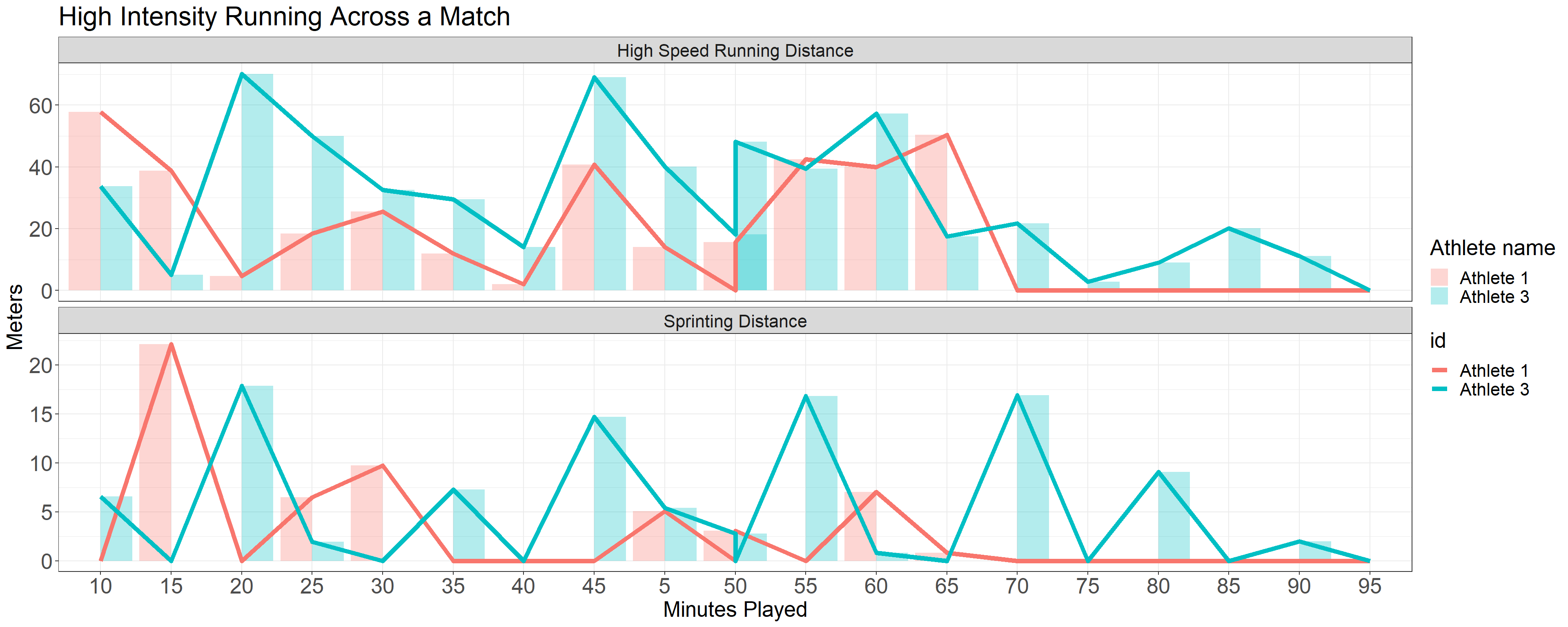 Thanks for reading. Hopefully you found it useful/interesting.
Lasse Ishøi
Head of Sport and Data Science at Football Club Nordsjælland (a Danish first tier club), and postdoc at Sports Orthopedic Research Center - Copenhagen (SORC-C)
My research interests include sport science, sport physiotherapy, and sport injuries.