Generate random sequence of bernoulli trials (e.g. coin flips)

rbinom(n=10, # 10 times
       size=1, # one trial (i.e. one throw)
       prob=0.3) # probability of success

##  [1] 1 1 0 0 1 0 1 0 0 1

rbinom(n=10, # 10 times
       size=100, # 100 trials (i.e. 100 throws) - output is then #number of successes
       prob=0.3) # probability of success

##  [1] 30 31 26 28 36 35 27 29 30 36

flips <- rbinom(n=100000, # 10 times
          size=10, #trials (i.e. n throws) - output is then #number of successes
          prob=0.5) # probability of success

hist(x = flips)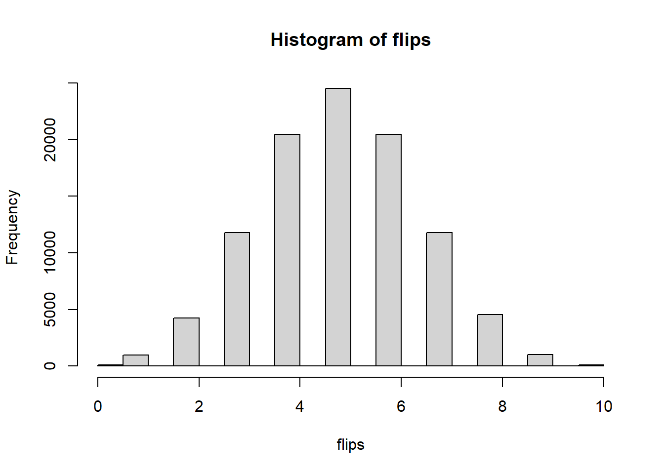

probability mass function

The probability Mass function of the binomial distribution is given by:

\[ P(X) = \frac{n!}{x!(n-x)!} p^x q^{n-x} \] Where:

• \(n\): number of trials (e.g., flips)
  
• \(p\): probability of success
  
• \(q = 1 - p\)
  
• Factorial: \(m!\) follows \(0! = 1, 1! = 1, 2! = 2 \times 1, 3! = 3 \times 2 \times 1\), etc.

The first part of the function is called The binomial coefficient, and it counts the number of ways x subjects can be drawn (choosen) from a population, n, and is expressed as n chooses x:

\[ \binom{n}{x} = \frac{n!}{x!(n-x)!} \] Where:

• \(n\): is the population
• \(x\): is the number drawn

#define parameters
x <- 5 # number of success
n <- 10 # size of population 
p <- 0.5 # probability of success

#Exact probability using the probability mass function

#define  function
binom_pmf <- function(x, n, p) {
  
  q <- 1-p
  
  binom_coef <- choose(n = n, k = x)
  
  binom_coef * p^x * q^(n-x)
  
}

binom_pmf(x = x, n = n, p = p)

## [1] 0.2460938

#Exact probability using in-built r function
dbinom(x = x, 
       size = n, 
       prob = p)

## [1] 0.2460938

#Simulated probability
mean(rbinom(n=100000,
        size=10,
        prob=0.5) == 5)

## [1] 0.24399

Calculate probability of at least x number of successes

#Exact probability
#Cumulative function - to find at least use the complementary probability
1- pbinom(q = 4, # 4 or less, (or at least five if using the complementary) 
       size = 10, # number of throws
       prob = 0.5) # probability

## [1] 0.6230469

#or use the lower.tail = FALSE (P[X > x])
pbinom(q = 4, # 4 or less, (or at least five if using the complementary) 
       size = 10, # number of throws
       prob = 0.5, lower.tail = FALSE) # probability

## [1] 0.6230469

#Simulated probability
mean(rbinom(n=100000,
        size=10,
        prob=0.5) >= 5)

## [1] 0.62189

#simulate several probabilities with different size using map
n <- c(100, 1000, 10000, 100000)


map_dbl(.x = n, ~mean(rbinom(n = .x,
        size=10,
        prob=0.5) >= 5))

## [1] 0.67000 0.59800 0.61750 0.62137

Expected value and variance

#Expected value
size <- 100
prob <- 0.8

#Simulation
mean(rbinom(n=10, # 10 times
       size=size, # 100 trials (i.e. 100 throws) - output is then #number of successes
       prob=prob)) # probability of success

## [1] 80.3

#Expected value rule
size*prob

## [1] 80

#variance

#simulation
var(rbinom(n=10, # 10 times
       size=size, # 100 trials (i.e. 100 throws) - output is then #number of successes
       prob=prob)) # probability of success

## [1] 11.15556

#Variance rule
size*prob*(1-prob)

## [1] 16

density <- function(x) {20/x^2}

integrate(density, lower = 10, upper = 20)

## 1 with absolute error < 1.1e-14

dbinom(2, 5, 0.9)

## [1] 0.0081